Position, Velocity, and Acceleration Lab
Partners: Madeline Walbert and Maeann Brougher
Date: 10/1/14
Purpose:
In this lab, we used two different methods to determine the five kinematic equations of a block going down a plane.
Date: 10/1/14
Purpose:
In this lab, we used two different methods to determine the five kinematic equations of a block going down a plane.
Theory:
|
The motion of an object can be described using the five kinematic quantities. These quantities can be derived using the four kinematic equations that are shown in Figure 1. The quantities associated with the motion of objects are:
Initial Velocity (Vi)= Starting rate at which an object changes its position. Final Velocity (Vf)= Ending rate at which an object changes its position. Acceleration (a)= Rate at which an object changes its velocity. Displacement (d)= Object's overall change in position. Time (t)= Measured period of which object moves. The kinematic quantities can also be derived by using position vs. time graphs, which are parabolas, and velocity vs. time graphs, which are linear. |
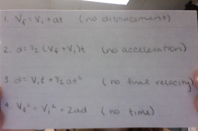
Figure 1: Four Kinematic Equations
|
Experimental Technique:
|
Method 1:
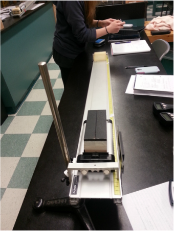
Figure 2: Plane
To find the five kinematic quantities of the designated interval, an earlier interval had to be calculated. The first interval started at the end of the block and ended at the start of the second interval. The second interval started further down from the block and ended a little above the end of the plane, which both points were marked by a piece of tape. Since there was already a pre-established ruler on the plane, the distance for the first interval was measured by subtracting the position of the end of the block from the position of the start of the second interval. A stopwatch was used to measure the time it took for the block to cover the first interval when released. Because the block is in a resting position, the inital velocity was known to be 0 m/s. Acceleration does not need to be calculated because it is not needed to solve the second interval. Final velocity, or the initial velocity of the second interval, was solved by using the equation V=d/t. Now for the second interval, time was again measured by releasing the block and using a stopwatch to see how long it took to cross the marked interval. Distance was found by looking at the ruler and subtracting the positions of the start of the interval from the end of the interval. Again, the final velocity for the second interval was found by using the equation V=d/t. In order to find acceleration, the equation Vf=Vi + at was used.
|
Method 2:
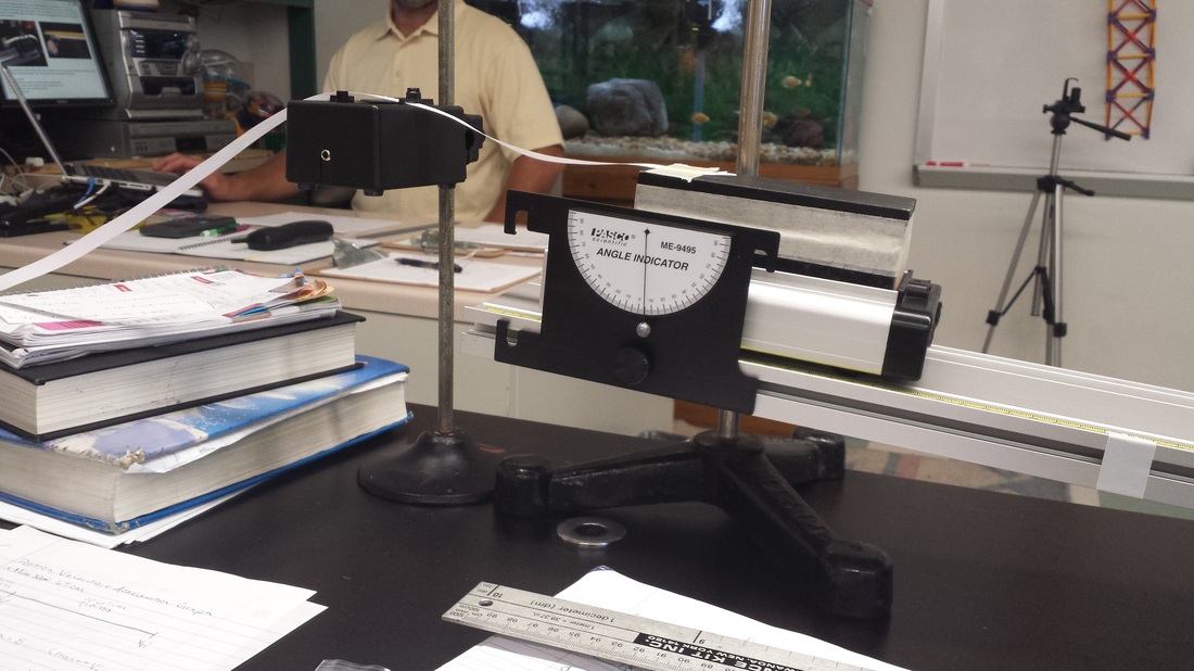
Figure 3: Ticker Tape Timer
For the second method, a ticker tape timer, shown above in Figure 3, was attached to the top of the plane to calculate the kinematic quantitites. First, the paper that goes through the ticker tape timer had to be marked to represent the interval being measured. The paper was then taped at the end to the block and passed through the timer. Next, the timer was set to 40 ticks/second and the block was released from the resting position. As the paper slid through the timer, the needle pushed on the carbon paper, producing black dots on the paper. At the end, the paper resulted in having 30 marks, or ticks, that got increasingly farther apart from each other.
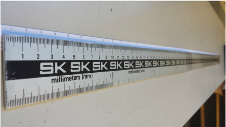
Figure 4: Measuring Ticks
After the paper had the marks from the ticker tape timer, the distances between each mark had to be measured using a ruler to find the positions of each point at each fraction of a second. This data was converted into an Excel chart. To find the velocity of each position, the equation V=d/t was used. To find the acceleration of each position, the equation a=V/t was used. This data was then used to form 3 graphs: Position Vs Time, Velocity Vs. Time, and Acceleration Vs. Time. Lastly, each graph received a best fit line and an equation of the line that demonstrated the accuracy of the measurements.
|
Data and Analysis:
Method 1:
Method 1:
|
For method 1, two intervals were calculated in order to find the five kinematic quantities. The distance of the first interval was found by subtracting 22cm from 30cm, resulting in 8cm. The time was found to be 0.57s using a stopwatch and the intial velocity is assumed to be 0m/s since the block is at resting position released. For the second interval, 30cm was subtracted from 97cm, resulting in 67cm and the stopwatch gave a time of 0.75s. To calculate the initial velocity of the second interval, or the final velocity of the first interval, the equation V=d/t was utilized. Meaning, the second initial velocity is 8cm/0.57s, equaling 14.0cm/s. The second final velocity was found using the same equation, so it was 67cm/0.75s, equaling 89.3cm/s. To find acceleration, the equation Vf= Vi + at was rearranged to be a= (Vf-Vi)/(t). Therefore, a= (89.3cm/s - 14.0cm/s)/(0.75s), or a= 100.4cm/s^2.
|
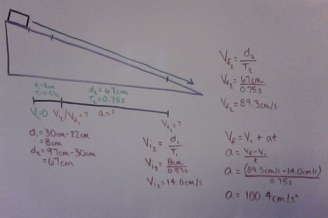
Figure 5: Method 1 Data
|
Method 2:
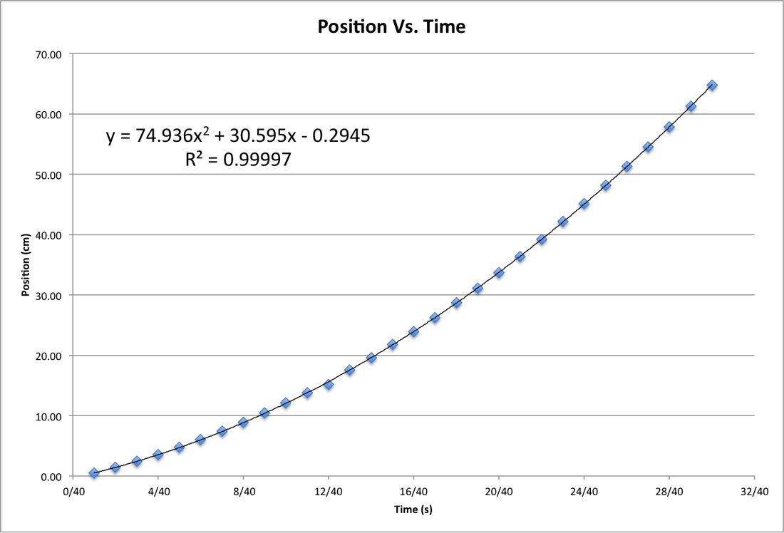
Figure 6: Postion Vs. Time Graph
The Position Vs. Time graph shows the relationship between each point's time compared to their position. It is a parabolic relationship and has the best accuracy compared to the other graphs.
|
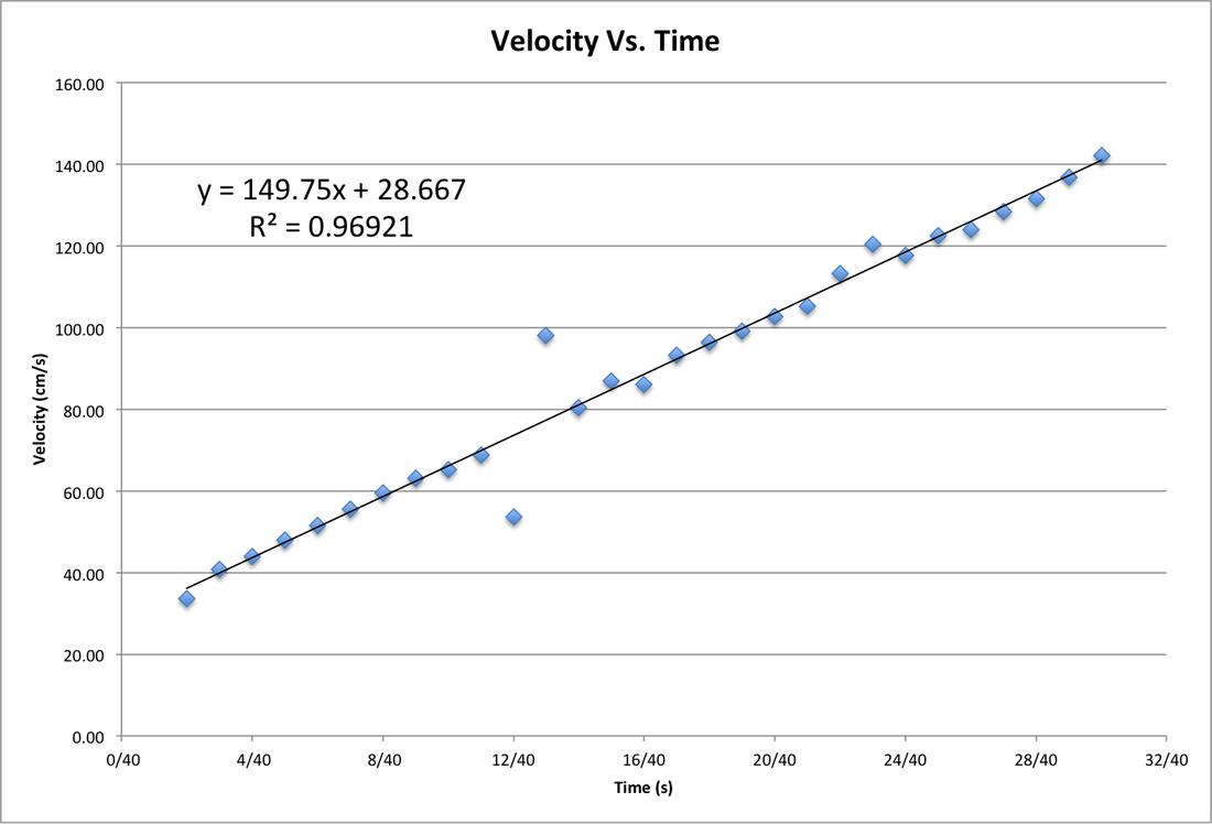
Figure 7: Velocity Vs. Time Graph
The Velocity Vs. Time graph demonstrates the relationship between the time of each point compared to their velocity at that time. This graph is considered linear and starts to have less accuracy, resulting in a little bit scattered presentation of information.
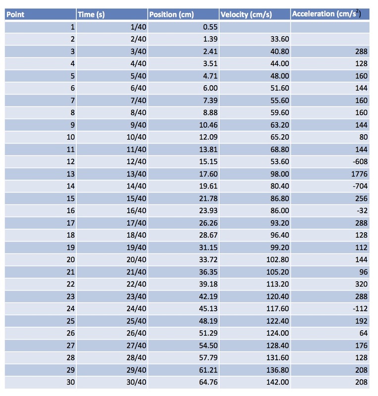
Figure 9: Graph's Data Table
The second method involved organizing the times, positions, velocities, and accelerations for each point into a data table that was later converted into 3 graphs.
|
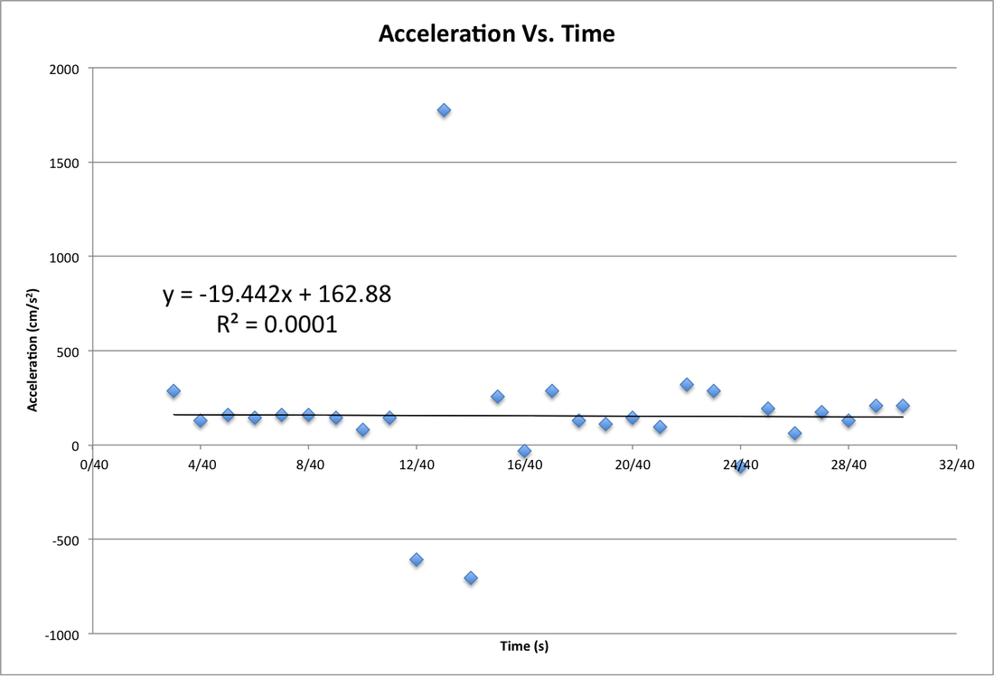
Figure 8: Acceleration Vs. Time Graph
The Acceleration Vs. Time graph shows the relationship between each point's time and acceleration at that specific time. This graph is completely scattered and cannot be used for any accurate measurements.
|
Conclusion:
In the lab, the five kinematic quantites, known as initial velocity, final velocity, time, distance, and acceleration, of an object sliding down a plane were discovered using two different methods. The first method involved timing the object crossing the designated interval and measuring the distance. The information was then utilized into equations to solve the remaining kinematic quantities. The second method involved using a ticker tape timer to find points to measure, which was then transformed into an Excel data table and 3 graphs: Position Vs. Time, Velocity Vs. Time, and Acceleration Vs. Time graphs.
One error that resulted in inaccurate measurements is reaction time. When using the stopwatch, there was a reaction time error because there was a delay with pressing the button at the exact moment, resulting in the wrong measurement. There was also measurement area when measuring the distance between each point with a ruler. Instead of starting at point 1, I should have started at point 0, which would have been where the interval started to where the first point was marked. But since that was not taken into account, the data is not as accurate as it should be. The Acceleration Vs. Time graph is especially inaccurate and cannot even be used to gather information because of the weak correlation between acceleration and time.
References:
Bowman, D. (n.d.). Lahs Physics. Lahs Physics. Retrieved October 15, 2014, from http://lahsphysics.weebly.com/
